Kicking Posterior
How Bayesian estimates quantify uncertainty in our data.
February 5, 2025
This is the second article in a three part series on Empirical Bayes inference for Kill Team Statistics. Checkout out the first article here.
It's been a minute since I wrote my last article. If I get any slower, I'll have to start calling them balance data slates.
Honestly, I didn’t expect anyone to read these articles beyond my wife (and she's content to limit conversations over imaginary space soldier statistics).
Anyway, let’s pick up where we left off, babe.
In the previous article, we covered Empirical Bayes point estimates and the concept of shrinkage. These updated averages provide a helpful summary for comparing exceptional factions with varying sample sizes (since low sample factions can produce unrealistic averages caused by noise and chance).
But it’s crucial to stress that Bayesian analysis accomplishes far more than adjusted averages. In Bayesian statistics, the complete estimate is not a single point. It’s a probability distribution called the Posterior.
The Posterior
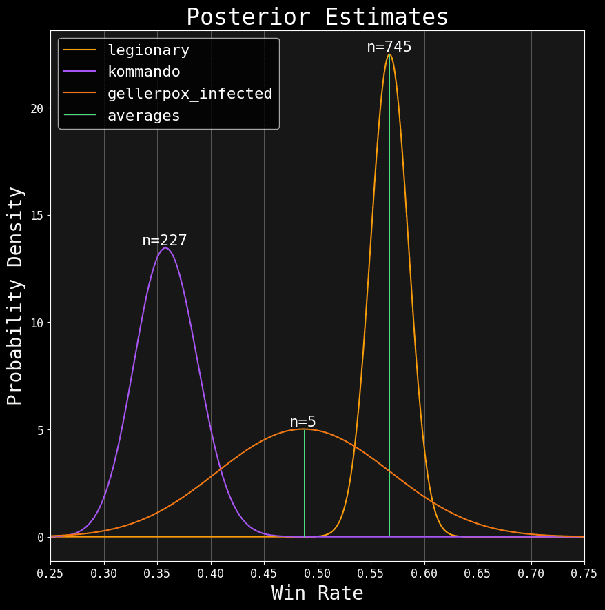
You're staring at three posteriors.
For this article, all estimates contain GT+ event data (At least 16 players with 4+ rounds) from the release of 3rd edition, 2024, up to (but not including) it's first data slate. Here's how you can read these distributions:
- The x-axis shows the range of possibilities for that faction's true win rate. Since win rate is a percentage, that range is always somewhere between
0and1. - The y-axis shows the probability density (i.e. how likely the corresponding win rate values are). Higher is better.
- Finally,
nshows the number of games for that faction.
Notice how factions with fewer games have a wide distribution, while those with more games have a narrow distribution. This means the fewer samples we have, the more uncertain we are (the probability distribution is stretched across a more extensive range of possible win rates). Meanwhile, the more samples we have, the more our certainty narrows (along with a higher likelihood of the remaining possible win rates).
Richard McElreath, in his excellent Bayesian Statistics course1, summarizes:
The posterior shape embodies the sample size.
Bayesian analysis is a framework for quantifying uncertainty. We don’t need to search for another method to calculate it; it’s baked in.
But this does mean averages alone can be insufficient. Check out those Gellerpox results! Their Bayesian average is 48.75%. But with only five games, there’s a high likelihood it isn't anywhere near 48.75%. With low samples, the average can be a misleading summary.
Fortunately, there are other ways to summarize posteriors. One way is to use Credible Intervals, a Bayesian version of the more commonly known Confidence Interval2.
Intervals of Cred
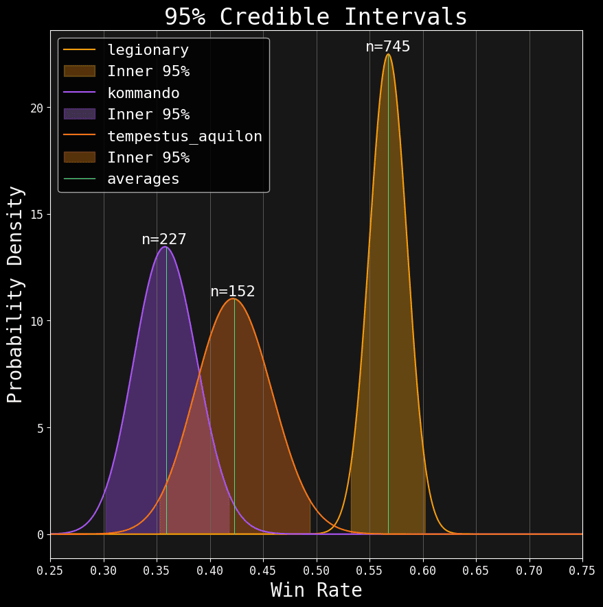
We'll swap out Gellerpox for Aquilions. Think of it as a warm up for getting 'declassified'.
In the above chart, the filled in portions of each estimate represent the 95% central mass (this mass leaves behind a 2.5% probability on both the left and right tails). The interval, in a credible interval, is merely the x-axis range that incorporates that central 95% mass. We call the lowest value the lower bound and the highest value the upper bound:
| Faction | Lower Bound | Upper Bound |
|---|---|---|
| Legionary | 53.24% | 60.19% |
| Aquilons | 35.27% | 49.38% |
| Kommandos | 30.19% | 41.77% |
However, look at how our estimate gets flattened in this translation. Our posterior is two-dimensional, but a credible interval is only one-dimensional. We lose all the nuance of the y-axis.
That nuance does matter; if you noticed, values closer to the average are more likely than values closer to the bounds of the interval (their y-axis value is higher). Like the average, credible intervals are just another summary value. They improve our perspective, but they still aren’t the full posterior.
I want to emphasize this point because, if you’re like me, your entire formal education in statistics was centered around significance testing; specifically, null hypothesis significance testing at a 0.05 significance level (the complement to a 95% confidence level).
This single-minded obsession has helped fill the internet with endless t-tests and ANOVA calculators, giving the impression that the Emperor’s finest delivered significance testing as an instrument for PURGING heretical data.
Significance testing is a tool for managing Type 1 Error; a tool that is particularly relevant in clinical or quality control settings3. It is not a catch-all method for declaring what data is valuable and what data is not.
Our goal with Kill Team win rates is to deliver an estimate with our data. There’s nothing special about 95%. It doesn't bring salvation any more than the averages do.
I find 95% intervals excessive for our usage. But hey, convention is convention; It doesn't hurt to keep it around in case the inquisition decides to show up. As a practical measure, I’ve added the 50% CI (which is the centermost half of the probable mass):
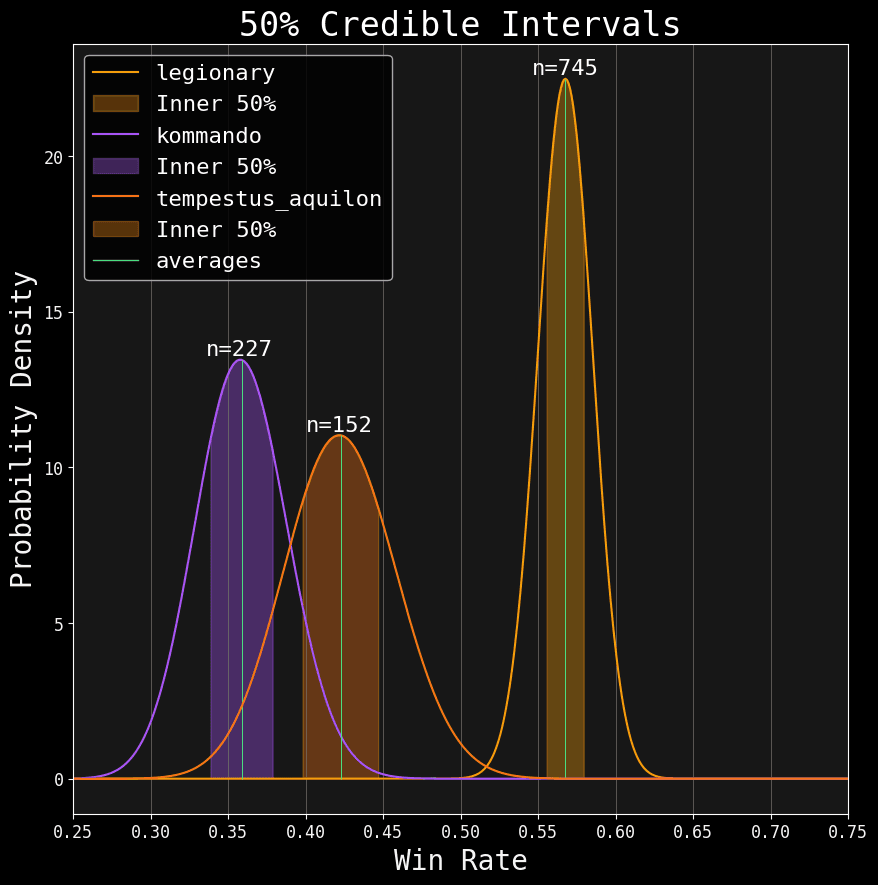
Central 50% mass of the posteriors.
50% CI is too narrow on it's own. But when combined with the 95%, it gives us a nice picture of our posteriors 😉. You can check out the values for all factions under the Spread tab on my analytics page.
Now, I know what you're thinking:
Smiles (or is it Lies?), surely there's more we can do with our posteriors!
Absolutely! Just as limitless as my dad jokes are, there are endless ways to analyze these bad bumps.
Goldilocks and the Three Probabilities
Most of you have heard of the Goldilocks Zone. The 45% - 55% zone James Workshop established as an acceptable range for win rates (in a way, this is James’ t-test). The idea is that any faction whose win rate exists outside this interval is considered over-turned or under-tuned (depending on whether you’re above or below this range, respectively).
Suppose we wanted to know the probability that a faction’s true win rate is above the 55% benchmark. We could look at the average, but we know that’s just a summary point. The complete estimate is in the posterior. So, to answer this question in a more principled way, we can do something like this:
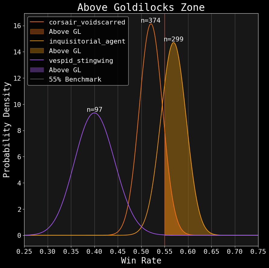
Let's plot my main faction: Corsairs; along with the despised Inquisition and some inferior xenos.
Notice the red line slicing through the posteriors. That is our 55% benchmark. I filled in the probability density above that mark. We can total each team's density like this:
| Faction | Above GL |
|---|---|
| Inquisition | 75.75% |
| Corsairs | 11.38% |
| Vespid | 0.79% |
Neat huh? Each of these percentages represent the probability that a faction is truly above 55%. We can do the same for the probability within the Goldilocks:
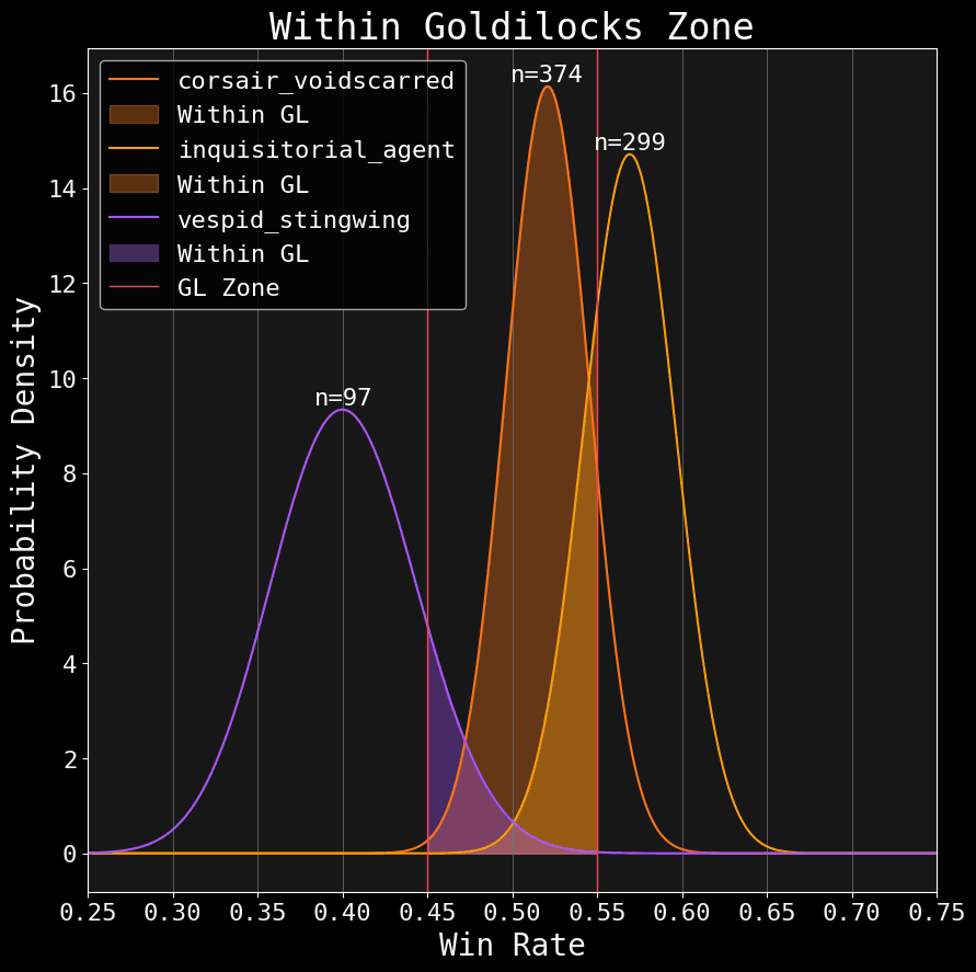
And of course, we can do the same for below the Goldilocks zone (notice how all three values add up to 100% for each team):
| Faction | Above GL | Within GL | Below GL |
|---|---|---|---|
| Inquisition | 75.75% | 24.25% | 0.00% |
| Corsairs | 11.83% | 87.96% | 0.21% |
| Vespid | 0.03% | 12.81% | 87.16% |
Once again, values for all factions can be found under the Spread tab on my analytics page.
Roll the Bones
One of the convenient things about Bayesian statistics is that, as war gamers, we can approach it in a similar way as dice math.
We all know a 3+ is better than a 5+. But hey, sometimes that injured guardsman gets lucky. Even worse, we’ve all burned a CP reroll on a 2+ only to whiff again.
Although probability can betray us, it's still a reliable guide for making calculated decisions. A good player knows dice math, but a great player seeks out the contexts where they can draw more value from their luck.
Consider our results: Inquisition has a 75.75% chance of being over the Goldilocks zone. At least, that’s what our mindless model tells us. So, is that outcome “significant?”
Well, we have a lot more context here than mere win rates, and I’m not just talking about other data like event wins and placing rates. We have a wealth of Domain Knowledge about these factions, information we’ve long held before anyone has played a single game. Unlike Mother Nature, James Workshop gave us the rule book.
Consider the tier lists produced by competitive players. They're quite popular, but some people dismiss them as “subjective."
Now, that's obviously true.
It's also misleading.
Yes, humans have biases. Yes, we should never treat opinions as hard science. But, this attitude is forgetting a crucial point. The faction rules endowed by Mr. Workshop are objective. We’re all constrained by the same rules (at least for any group capable of reading). Experienced and reasonable people can draw conclusions from these rules.
Given what we knew about these rules, as they existed when the new edition was released, I’d call 75.75% on Inquisition being over-tuned a safe bet. You can save your CP.
This diatribe may sound self-defeating coming from a self-appointed "Stats Guy," but I find it stupid to pit perfectly valid sources of information against each other as though they are locked in a blood feud. Domain knowledge and data both matter.
The data grounds us: It fights against our bias and blind spots while providing nuance and precision. Yet, domain knowledge provides the context for interpreting data. Without domain knowledge, data is worthless. Anyone who claims “The data is all we need!” is just hiding assumptions they aren’t telling you.
Butts. There, I said it.
Uncertainty is a fact of life. Carefully recognizing its scope and influence is vital to making informed judgments. If we exaggerate our uncertainty, we will end up discarding meaningful information. But if we ignore uncertainty, we become dogmatists. Both paths are a form of ignorance that would make the Imperium proud.
In statistics, quantifying uncertainty between the observed data and our subject of interest is called Inference (which is what we have been doing in these articles).
My next article will discuss inference more explicitly as it applies to competitive Kill Team. Then, we'll see how to leverage our estimates to produce a statistically driven tier list.
Thanks for the read! 🧐🥃
Footnotes:
Here are some essential differences between confidence and credible intervals:
- Credible intervals can benefit from our prior (which I mentioned in the last article); this helps constrain the interval into a more realistic range at smaller sample sizes.
- Credible intervals use an intuitive understanding of probability. Namely, if I say I have a
credible interval of
95%, I mean there’s a95%chance the true value exists within that interval range. - Not all values within the credible interval are equally likely. This is also the case with confidence intervals, in that not all values have equal confidence.